Distance Metrics

Euclidean & Cosine

Euclidean distance is the straight line distance between points, while Cosine Similarity is the angle between these two points.

from scipy.spatial.distance import euclidean, cosine

euclidean([1,2],[1,3])
# 1
cosine([1,2],[1,3])
# 0.010050506338833642

Mahalanobis Distance

Mahalonobis distance is the distance between a point and a distribution, not between two distinct points. Therefore, it is effectively a multivariate equivalent of the Euclidean distance. More here.

Type	Desc
x	vector of the observation (row in a dataset)
m	vector of mean values of independent variables (mean of each column)
C^(-1)	inverse covariance matrix of independent variables

Multiplying by the inverse covariance (correlation) matrix essentially means dividing the input with the matrix. This is so that if features in your dataset are strongly correlated, the covariance will be high. Dividing by a large covariance will effectively reduce the distance.

While powerful, its use of correlation can be detrimantal when there is multicollinearity (strong correlations among features).

import pandas as pd
import numpy as np
from scipy.spatial.distance import mahalanobis

def mahalanobisD(normal_df, y_df):
    # calculate inverse covariance from normal state
    x_cov = normal_df.cov()
    inv_cov = np.linalg.pinv(x_cov)

    # get mean of normal state df
    x_mean = normal_df.mean()

    # calculate mahalanobis distance from each row of y_df
    distanceMD = []
    for i in range(len(y_df)):
        MD = mahalanobis(x_mean, y_df.iloc[i], inv_cov)
        distanceMD.append(MD)

    return distanceMD

Dynamic Time Warping

If two time series are identical, but one is shifted slightly along the time axis, then Euclidean distance may consider them to be very different from each other. DTW was introduced to overcome this limitation and give intuitive distance measurements between time series by ignoring both global and local shifts in the time dimension.

DTW is a technique that finds the optimal alignment between two time series, if one time series may be “warped” non-linearly by stretching or shrinking it along its time axis.

Dynamic time warping is often used in speech recognition to determine if two waveforms represent the same spoken phrase. In a speech waveform, the duration of each spoken sound and the interval between sounds are permitted to vary, but the overall speech waveforms must be similar.

There is a faster implementation of DTW called Fast DTW.

The result is DTW is such that if two time-series are identical, the DTW distance is 0, else any difference will be more than 0.

import numpy as np
from scipy.spatial.distance import euclidean
from fastdtw import fastdtw

x = np.array([[1,1], [2,2], [3,3], [4,4], [5,5]])
y = np.array([[2,2], [3,3], [4,4]])
distance, path = fastdtw(x, y, dist=euclidean)
print(distance)

# 2.8284271247461903

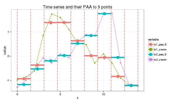
Symbolic Aggregate approXimation

SAX, developed in 2007, compares the similarity of two time-series patterns by slicing them into horizontal & vertical regions, and comparing between each of them. This can be easily explained by 4 charts shown below.

There are obvious benefits using such an algorithm, for one, it will be very fast as pattern matching is aggregated. However, the biggest downside is that both time-series signals have to be of same time-length.

Both signals are overlayed

Then normalised.

The chart is then sliced by various timeframes, Piecewise Aggregate Approximation, and each slice is compared between the two signals independently.

Each signal value, i.e., y-axis is then sliced horizontally into regions, and assigned an alphabet.

Lastly, we use a distance scoring metric, through a fixed lookup table to easily calculate the total scores between each pair of PAA.

E.g., if the PAA fall in a region or its immediate adjacent one, we assume they are the same, i.e., distance = 0. Else, a distance value is assigned. The total distance is then computed to derice a distance metric.

For this instance:

• SAX transform of ts1 into string through 9-points PAA: “abddccbaa”
• SAX transform of ts2 into string through 9-points PAA: “abbccddba”
• SAX distance: 0 + 0 + 0.67 + 0 + 0 + 0 + 0.67 + 0 + 0 = 1.34

This is the code from the package saxpy. Unfortunately, it does not have the option of calculating of the sax distance.

import numpy as np
from saxpy.znorm import znorm
from saxpy.paa import paa
from saxpy.sax import ts_to_string
from saxpy.alphabet import cuts_for_asize

def saxpy_sax(signal, paa_segments=3, alphabet_size=3):
  sig_znorm = znorm(signal)
  sig_paa = paa(sig_znorm, paa_segments)
  sax = ts_to_string(sig_paa, cuts_for_asize(alphabet_size))
  return sax

sig1a = saxpy_sax(sig1)
sig2a = saxpy_sax(sig2)

Another more mature package is tslearn. It enables the calculation of sax distance, but the sax alphabets are set as integers instead.

from tslearn.piecewise import SymbolicAggregateApproximation

def tslearn_sax(sig1, sig2, n_segments, alphabet_size):

  # Z-transform, PAA & SAX transformation
  sax = SymbolicAggregateApproximation(n_segments=n_segments,
                                       alphabet_size_avg=alphabet_size)
  sax_data = sax.fit_transform([sig1_n,sig2_n])

  # distance measure
  distance = sax.distance_sax(sax_data[0],sax_data[1])

  return sax_data, distance

# [[[0]
#   [3]
#   [3]
#   [1]]

#  [[0]
#   [1]
#   [2]
#   [3]]]

# 1.8471662549420924