Classification
Supervised classification is done when the label is a categorical variable.
KNN
K-Nearest Neighbours is computed from a simple majority vote of the nearest neighbors of each point: a query point is assigned the data class which has the most representatives within the nearest neighbors of the point.
| Hyperparameter(s) | Desc |
|---|---|
| n_neighbors | no. nearest neighbours from a point to assign a class. default 5 |
| metric | default=’minkowski’, i.e. euclidean |
import pandas as pd
import numpy as np
from sklearn.cross_validation import train_test_split
from sklearn.neighbors import KNeighborsClassifier

X_train, X_test, y_train, y_test = train_test_split(X, y, random_state=0)
knn = KNeighborsClassifier(n_neighbors = 5)
knn.fit(X_train, y_train)
knn.score(X_test, y_test)
# 0.53333333333333333
Naive Bayes
Naive Bayes is a probabilistic model using the Bayes' theorem. Features are assumed to be independent of each other in a given class (hence naive). This makes the math very easy. E.g., words that are unrelated multiply together to form the final probability.
There are 5 variants of Naive Bayes in sklearn. Bernouli and Multinomial models are commonly used for sparse count data like text classification. The latter normally works better. Gaussian model is used for high-dimensional data.
| Hyperparameter(s) | Desc |
|---|---|
| alpha | smoothing (generalisation) parameter (default 1.0) |

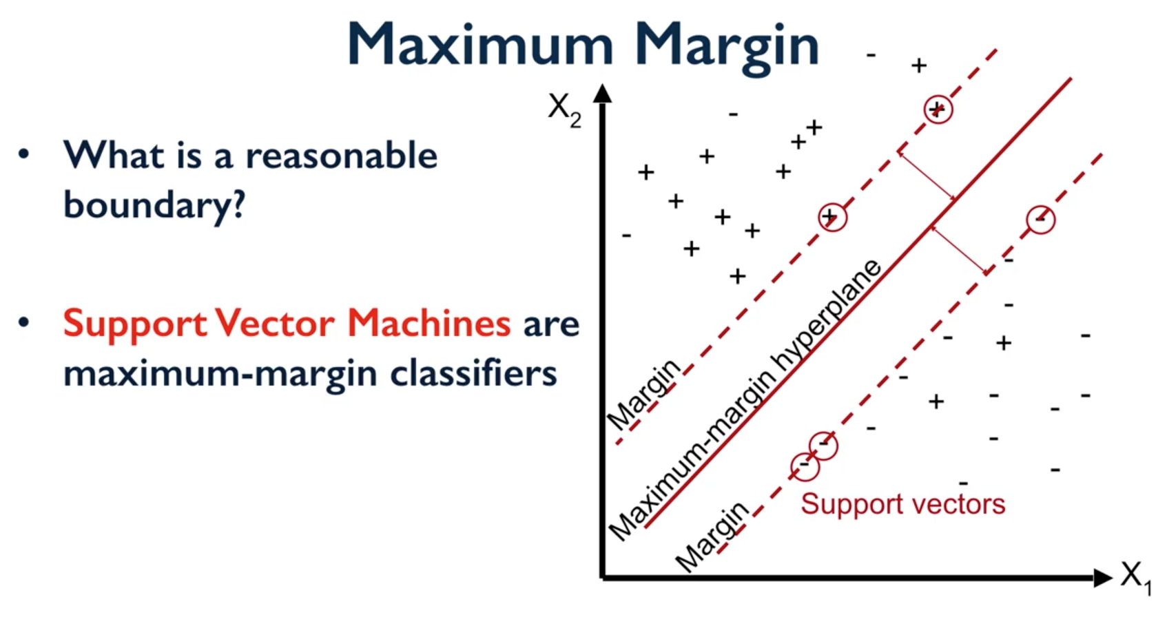
Support Vector Machines
Support Vector Machines (SVM) involves locating the support vectors of two boundaries to find a maximum tolerance hyperplane.
| Key hyperparameter(s) | Desc |
|---|---|
| C | lower C more L2 regularization |
| kernel | linear or radial basis function (rbf) |
| gamma | from v0.22, gamma is auto or scaled, rather than a float |

from sklearn.preprocessing import MinMaxScaler
scaler = MinMaxScaler()
X_train_scaled = scaler.fit_transform(X_train)
X_test_scaled = scaler.transform(X_test)

clf = SVC(kernel='rbf', C=10).fit(X_train_scaled, y_train)
If we require linear SVM, we should use LinearSVC with its flexibility of regularization and loss functions, together with faster compute time for large datasets.
from sklearn.svm import LinearSVC

clf = LinearSVC(penalty='l2', loss='squared_hinge', C=1.0)
Logistic Regression
While it is a type of regression, it only outputs a binary value hence it is considered a classification model.
| Key hyperparameter(s) | Desc |
|---|---|
| penalty | l1/l2/elasticnet |
| C | lower C more regularization |

from sklearn.linear_model import LogisticRegression

clf = LogisticRegression(C=100).fit(X_train, y_train)
acc_train = clf.score(X_train, y_train)
acc_test = clf.score(X_test, y_test)
Decision Tree
Uses gini index (default) or entropy to split the data at binary level.
Strengths: Can select a large number of features that best determine the targets.
Weakness: Tends to overfit the data as it will split till the end. Pruning (using max_depth & min_samples_leaf) can be done to remove the leaves to prevent overfitting. Small changes in data can lead to different splits. Not very reproducible for future data (tree ensemble methods are better).
| Key hyperparameter(s) | Desc |
|---|---|
| max_depth | The maximum depth of the tree |
| min_samples_leaf | The minimum number of samples required before splitting |
import pandas as pd
import numpy as np
from sklearn.tree import DecisionTreeClassifier

X_train, y_train, x_test, y_test = \
train_test_split(predictor, target, test_size=0.25)

clf = DecisionTreeClassifier()
model = clf.fit(X_train, y_train,
                max_depth=4, min_samples_leaf=8, max_features)

predictions = model.predict(x_test)
accuracy = sklearn.metrics.accuracy_score(y_test, predictions)
print(accuracy)
# 0.973684210526

# Feature importance
f_impt= pd.DataFrame(model.feature_importances_, index=df.columns[:-2])
f_impt = f_impt.sort_values(by=0, ascending=False)
f_impt.columns = ['feature importance']
print(f_impt)
# petal width (cm)      0.952542
# petal length (cm)     0.029591
# sepal length (cm)     0.017867
# sepal width (cm)      0.000000
Viewing the decision tree requires installing of the two packages conda install graphviz & conda install pydotplus.
from sklearn.externals.six import StringIO
from IPython.display import Image
from sklearn.tree import export_graphviz
import pydotplus

dot_data = StringIO()
export_graphviz(dtree, out_file=dot_data,
                filled=True, rounded=True,
                special_characters=True)
graph = pydotplus.graph_from_dot_data(dot_data.getvalue())
Image(graph.create_png())

Tree Ensembles
Random Forest
An ensemble of decision trees. Used to be one of the most popular tree classifiers. But now generally superceded by other variants like XGBoost, LightGBM etc.
Each decision tree is random, introduced through bootstrap (aka, bagging), i.e. sample of size N is created by just repeatedly picking one of the N dataset rows at random with replacement, as well as random feature splits, i.e., when picking the best split for a node, instead of finding the best split across all possible features (decision tree), a random subset of features is chosen and the best split is found within that smaller subset of features
As a result of this randomness, the model is very generalized.
| Key hyperparameter(s) | Desc |
|---|---|
| n_estimators | no. decision trees |
| max_features | max random features to split a leaf node |
import pandas as pd
import numpy as np
from sklearn.ensemble import RandomForestClassifier
from sklearn.cross_validation import train_test_split
import sklearn.metrics

train_feature, test_feature, train_target, test_target = \
train_test_split(feature, target, test_size=0.2)


clf = RandomForestClassifier(n_estimators=100, n_jobs=4, verbose=3)
model = clf.fit(train_feature, train_target)

predictions = model.predict(test_feature)
accuracy = sklearn.metrics.accuracy_score(y_test, predictions)
print(accuracy)
0.823529411765

# feature importance
f_impt= pd.DataFrame(model.feature_importances_, index=df.columns[:-2])
f_impt = f_impt.sort_values(by=0,ascending=False)
f_impt.columns = ['feature importance']
print(f_impt)
To see how many decision trees are minimally required make the accuracy plateau.
import numpy as np
import matplotlib.pylab as plt
import seaborn as sns
%matplotlib inline

trees=range(100)
accuracy=np.zeros(100)

for i in range(len(trees)):
  clf=RandomForestClassifier(n_estimators= i+1)
  model=clf.fit(train_feature, train_target)
  predictions=model.predict(test_feature)
  accuracy[i]=sklearn.metrics.accuracy_score(test_target, predictions)

plt.plot(trees,accuracy)

Gradient Boosting
The general idea of most boosting methods is to train predictors sequentially, each trying to correct its predecessor. Gradient boosting tries to fit the new predictor to the residual errors made by the previous predictor.
Built in a non-random way, to create a model that makes fewer and fewer mistakes as more trees are added. Once the model is built, making predictions with a gradient boosted tree models is fast and doesn’t use a lot of memory.
| Key hyperparameter(s) | Desc |
|---|---|
| n_estimators | no. of boosting stages to perform. Gradient boosting is fairly robust to over-fitting so a large number usually results in better performance. |
| learning_rate | controls how hard each tree tries to correct mistakes from previous round. Higher learning rate, more complex trees. |
XGBoost
XGBoost or eXtreme Gradient Boosting, is a form of gradient boosted decision trees is that designed to be highly efficient, flexible and portable.
from xgboost import XGBClassifier
from sklearn.model_selection import train_test_split
from sklearn.metrics import accuracy_score

X_train, X_test, y_train, y_test = train_test_split(X, Y, random_state=0)

model = XGBClassifier()
model.fit(X_train, y_train)

y_pred = model.predict(X_test)
predictions = [round(value) for value in y_pred]

accuracy = accuracy_score(y_test, predictions)
print("Accuracy: %.2f%%" % (accuracy * 100.0))
LightGBM
LightGBM (Light Gradient Boosting) is a lightweight version of gradient boosting developed by Microsoft. It has similar performance to XGBoost but touted to run much faster than it.
import lightgbm

X_train, X_test, y_train, y_test = \
train_test_split(x, y, test_size=0.2, random_state=42, stratify=y)

# Create the LightGBM data containers
train_data = lightgbm.Dataset(X_train, label=y)
test_data = lightgbm.Dataset(X_test, label=y_test)

parameters = {
  'application': 'binary',
  'objective': 'binary',
  'metric': 'auc',
  'is_unbalance': 'true',
  'boosting': 'gbdt',
  'num_leaves': 31,
  'feature_fraction': 0.5,
  'bagging_fraction': 0.5,
  'bagging_freq': 20,
  'learning_rate': 0.05,
  'verbose': 0
}

model = lightgbm.train(parameters,
                      train_data,
                      valid_sets=test_data,
                      num_boost_round=5000,
                      early_stopping_rounds=100)
CatBoost
Category Boosting has high performances compared to other popular models, and does not require conversion of categorical values into numbers. It is said to be even faster than LighGBM, and allows model to be ran using GPU.
TabNet
This is a neural network architecture developed by Google in 2019, said to provide better performance than tree ensembles and also better explainability comparable to decision trees.
The following two sites from towardsdatascience & google blog explains it well.
Use pip install pytorch-tabnet to use the pytorch implementation of this network.
Here's an example of how to train the model from its documentation.
from pytorch_tabnet.tab_model import TabNetClassifier, TabNetRegressor

clf = TabNetClassifier()  #TabNetRegressor()
clf.fit(
  X_train, Y_train,
  eval_set=[(X_valid, y_valid)]
)
preds = clf.predict(X_test)
Voting
The idea behind the VotingClassifier is to combine conceptually different machine learning classifiers and use a majority vote (hard vote) or the average predicted probabilities (soft vote) to predict the class labels. Such a classifier can be useful for a set of equally well performing model in order to balance out their individual weaknesses.
Tree ensembles is an example of a majority voting model.
Stacking
Stacked generalization is a method for combining estimators to reduce their biases. More precisely, the predictions of each individual estimator are stacked together and used as input to a final estimator to compute the prediction. This final estimator is trained through cross-validation.
The fundamental difference between voting and stacking is how the final aggregation is done. In voting, user-specified weights are used to combine the classifiers whereas stacking performs this aggregation by using a blender/meta classifier.