Model Evaluation

A large portion of model evaluation is derived from sklearn. Do check out their documentation for their latest APIs.

Classification

The various commonly used evaluation metrics for classification problems are as listed.

Type	Formula	Desc	Example
Accuracy	TP + TN / (TP + TN + FP + FN)	Get % TP & TN	We never use accuracy on its own
Precision	TP / (TP + FP)	High precision means it is important to filter off the any false positives.	Spam removal
Recall	TP / (TP + FN)	High recall means to get all positives (TP + FN) despite having some false positives.	Tumour detection
F1	2*((Precision * Recall) / (Precision + Recall))	Harmonic mean of precision & recall	-

from sklearn.metrics import (accuracy_score, precision_score, 
                             recall_score, f1_score)
from statistics import mean


accuracy = accuracy_score(y_test, y_predicted)
precision = precision_score(y_test, y_predicted)
recall = recall_score(y_test, y_predicted)
f1 = f1_score(y_test, y_predicted)


# for multiclass classification
# we need to compute their mean

precision = mean(precision_score(y_test, y_predicted, average=None))
recall = mean(recall_score(y_test, y_predicted, average=None))
f1 = mean(f1_score(y_test, y_predict, average=None))

Confusion Matrix

The confusion matrix is the most important visualization to plot for a classification evaluation. It shows the absolute breakdown of each prediction to see if they are in the correct class; and is usually in a heatmap for better clarity.

import matplotlib.pyplot as plt
from sklearn.metrics import plot_confusion_matrix

confusion = plot_confusion_matrix(model, X_test, y_test, cmap=plt.cm.Blues)
plt.savefig("logs/confusion_metrics.png")

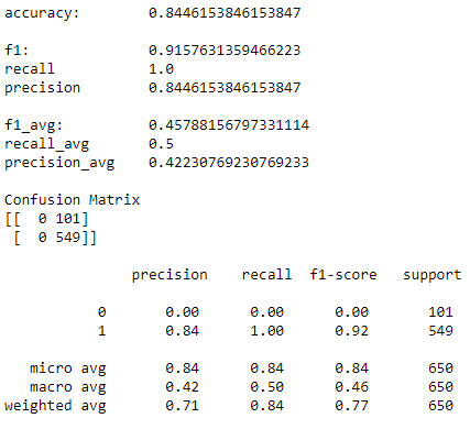
Classification Report

We can use the classification report to show details of precision, recall & f1-scores for each class.

from sklearn.metrics import classification_report

cls_report = classification_report(y_test, y_predict)
print(cls_report)

Precision-Recall Curve

From sklearn, the precision-recall curve shows the tradeoff between precision and recall for different threshold.

A high area under the curve represents both high recall and high precision, where high precision relates to a low false positive rate, and high recall relates to a low false negative rate.

from sklearn.metrics import precision_recall_curve
from sklearn.metrics import plot_precision_recall_curve
import matplotlib.pyplot as plt

average_precision = average_precision_score(y_test, y_score)
disp = plot_precision_recall_curve(classifier, X_test, y_test)
disp.ax_.set_title('2-class Precision-Recall curve: '
                   'AP={0:0.2f}'.format(average_precision))

sklearn documentation

ROC Curve

The receiver operating characteristic (ROC) curve evaluates the performance of a classifier by plotting the True Positive Rate vs the False Positive Rate. The metric, area under curve (AUC) is used. The higher the AUC, the better the model is.

The term came about in WWII where this metric is used to determined a receiver operator’s ability to distinguish false positive and true postive correctly in the radar signals.

from sklearn.metrics import plot_roc_curve

svc_disp = plot_roc_curve(svc, X_test, y_test)
plt.show()

sklearn documentation

---

Regression

For regression problems, the response is always a continuous value, so it requires a different set of evaluation metrics. This website gives an excellent description on all the variants of errors metrics, which are briefly summarised below.

Type	Desc
R-Squared	Percentage of variability of dataset that can be explained by the model
MSE (Mean Squared Error)	Squaring then getting the mean of all errors (so change negatives into positives)
RMSE (Squared Root of MSE)	So that it gives back the error at the same scale (as it was initially squared)
MAE (Mean Absolute Error)	For negative errors, convert them to positive and obtain all error means
RMSLE (Root Mean Square Log Error)	Helps to reduce the effects of outliers compared to RMSE

The RMSE result will always be larger or equal to the MAE. However, if all of the errors have the same magnitude, then RMSE=MAE.

Since the errors were squared before they are averaged, the RMSE gives a relatively high weight to large errors. This means the RMSE should be more useful when large errors are particularly undesirable.

import numpy as np
from sklearn.metrics import mean_squared_error
from sklearn.metrics import mean_absolute_error

model = RandomForestRegressor(n_estimators= 375)
model3 = model.fit(X_train, y_train)
fullmodel = model.fit(predictor, target)

# R2
r2_full = fullmodel.score(predictor, target)
r2_train = model3.score(X_train, y_train)
r2_test = model3.score(X_test, y_test)

# get predictions
y_predicted_total = model3.predict(predictor)
y_predicted_train = model3.predict(X_train)
y_predicted_test = model3.predict(X_test)

# get MSE
MSE_total = mean_squared_error(target, y_predicted_total)
MSE_train = mean_squared_error(y_train, y_predicted_train)
MSE_test = mean_squared_error(y_test, y_predicted_test)

# get RMSE by squared root
RMSE_total = np.sqrt(MSE_total)
RMSE_train = np.sqrt(MSE_train)
RMSE_test = np.sqrt(MSE_test)

# get MAE
MAE_total = mean_absolute_error(target, y_predicted_total)
MAE_train = mean_absolute_error(y_train, y_predicted_train)
MAE_test = mean_absolute_error(y_test, y_predicted_test)

RMSLE is a very popular evaluation metric in data science competitions. More about it in this medium article.

def rmsle(y, y0):
    assert len(y) == len(y0)
    return np.sqrt(np.mean(np.power(np.log1p(y)-np.log1p(y0), 2)))